Kinetic Modeling and Energy Optimization of Biogas Production from Slaughterhouse Waste in Forest Guinea

Faya Maurice Yombouno; Toha François Lihonou; Ansoumane Sakouvogui; Ibrahima Bayo; Nakany Camara; Salifou Tera

doi:doi:10.11648/j.sjee.20261404.11

Review Article |

| Peer-Reviewed

Kinetic Modeling and Energy Optimization of Biogas Production from Slaughterhouse Waste in Forest Guinea

Faya Maurice Yombouno^*

, Toha François Lihonou

, Ansoumane Sakouvogui

, Ibrahima Bayo

, Nakany Camara, Salifou Tera

Published in Science Journal of Energy Engineering (Volume 14, Issue 4)

Received: 23 September 2026 Accepted: 4 October 2026 Published: 26 October 2026

Views: Downloads:

Download PDF

Share This Article

Twitter
Linked In
Facebook

Abstract

Anaerobic digestion of slaughterhouse waste can mitigate pollution while supplying locally usable energy. Final biogas volume alone, however, does not define a rational operating time. This study modeled daily kinetics from four experimental loads monitored for 40 days in N’Zérékoré: diluted rumen content (D1), blood (D2), rumen content-pig slurry (D3), and a more concentrated rumen-content treatment (D4). First-order, modified Gompertz, logistic, and Cone models were fitted by nonlinear least squares to daily increments and compared using corrected Akaike information criterion, RMSE, MAE, , and residual diagnostics. Fitting uncertainty was assessed using 1,000 moving-block bootstrap repl icates. An operational threshold,, was defined as the modeled time required to recover 90% of the biogas energy observed on day 40. Recalculated cumulative volumes were 2,432, 3,415, 795, and 2,492 mL per experimental load for (D1)-(D4). The Cone model was selected for (D1) and (D4), whereas the modified Gompertz model best described (D2) and (D3). Estimated values were 16.84, 19.39, 35.80, and 28.53 days, respectively. Using methane fractions reported in the source study and a methane lower heating value of 9.94 kWh/, apparent gross energies were 15.92, 23.17, 4.51, and 16.31 Wh per load. (D2) combined the highest total energy with an energy productivity of 1.075 Wh/day at . The proposed operating times would shorten digester occupancy by 57.9%, 51.5%, 10.5%, and 28.7% relative to a fixed 40-day cycle. These estimates provide a numerical decision aid for cycle duration, rather than causal optimization of operating variables, because the dataset includes no biological replicates, blank controls, or factorial design.

Published in	Science Journal of Energy Engineering (Volume 14, Issue 4)
DOI	10.11648/j.sjee.20261404.11
Page(s)	98-111
Creative Commons	This is an Open Access article, distributed under the terms of the Creative Commons Attribution 4.0 International License (http://creativecommons.org/licenses/by/4.0/), which permits unrestricted use, distribution and reproduction in any medium or format, provided the original work is properly cited.
Copyright	Copyright © The Author(s), 2026. Published by Science Publishing Group

Keywords

Anaerobic Digestion, Slaughterhouse Waste, Biogas, Modified Gompertz, Cone Model, Energy Optimization, Forest Guinea

1. Introduction

The transition toward low-carbon energy systems increasingly relies on technologies capable of producing renewable energy while sustainably managing organic waste. Anaerobic digestion (AD) has become a mature technology in this context, converting biodegradable organic matter into biogas composed mainly of methane (CH₄) and carbon dioxide (CO₂), while reducing the pollutant load of waste and generating a digestate that can be used in agriculture (

[1, 2]

. The process relies on a sequence of microbiological processes hydrolysis, acidogenesis, acetogenesis, and methanogenesis—whose overall efficiency depends on the balance among these stages and on physicochemical conditions

[3]

In sub-Saharan Africa, AD is of particular interest because traditional biomass remains a major energy source and waste from agriculture, livestock production, and agro-industry is abundant. In Guinea, particularly in Forest Guinea, pressure on wood and charcoal remains high for household energy supply, while agricultural and slaughterhouse activities generate large amounts of organic matter that are still insufficiently valorized. Converting these wastes into biogas would provide multiple benefits: renewable energy production, reduction of environmental nuisances, and lower pressure on woody resources.

Slaughterhouse waste is among the most attractive organic resources from an energy perspective because of its high biodegradable-matter content. It consists of blood, rumen content, fecal matter, fats, organic tissues, and wastewater, with substantial compositional variability. Protein and lipid-rich fractions have high methanogenic potential

[4, 5]

. In

[4]

, authors showed that slaughterhouse waste has substantial methane potential, but its valorization requires precise control of digestion dynamics. High organic loading is both an energy advantage and a source of instability: protein degradation generates ammoniacal nitrogen, whereas lipid hydrolysis produces long-chain fatty acids (LCFAs) that may inhibit methanogenesis at high concentrations

[4, 6]

. Lipid-rich wastes can therefore produce large amounts of methane but may experience inhibition when organic loading exceeds microbial adaptation capacity. In

[5]

, authors observed high methane yields with transient LCFA accumulation, underscoring that final methane volume alone is insufficient to characterize process performance.

Slaughterhouse wastewater, characterized by high concentrations of organic matter, proteins, and lipids, has a high pollution potential if discharged untreated

[7, 8]

. Its treatment by AD provides a dual benefit: pollution reduction and energy recovery. Several studies

[7, 9]

have confirmed the feasibility of anaerobic treatment of slaughterhouse effluents, particularly using UASB reactors or anaerobic filters, reinforcing the relevance of anaerobic digestion in contexts with limited waste-management infrastructure.

AD performance nevertheless depends on many parameters: temperature, pH, organic loading, dry matter, inoculum/substrate ratio, nutrient availability, and retention time

[10, 11]

. Maintaining conditions favorable to methanogenic activity is crucial because microorganisms are sensitive to pH variations, accumulation of volatile fatty acids, ammonia, and certain sulfur compounds

[6]

. An increase in organic loading does not necessarily result in a proportional increase in methane production, especially when inhibition occurs.

The diversity and heterogeneity of slaughterhouse waste, whose constituents (blood, rumen content, fats, wastewater) have different degradation dynamics, complicate its valorization. Carbohydrates, proteins, and lipids follow distinct metabolic pathways and influence microbial population dynamics. Two substrates with similar methanogenic potential may have very different start-up times and production rates. Thus, final biogas volume alone does not indicate the optimal digester operating duration.

Co-digestion, which consists of treating several organic materials together, makes it possible to exploit substrate complementarity in terms of C/N ratio, biodegradability, buffering capacity, and nutrient availability

[12, 13]

. It may also dilute certain inhibitors and stabilize the microbial system. However, synergistic effects are not systematic and vary according to substrate type and proportion

[14]

. It is therefore necessary to experimentally evaluate different loads rather than assume that a mixture necessarily produces more methane than the individual substrates.

Biochemical methane potential (BMP) tests are reference methods for determining substrate biodegradability and methanogenic potential

[15-17]

. They monitor cumulative methane production under controlled conditions and estimate the maximum amount produced per unit of organic matter. However, results depend on inoculum type, inoculum/substrate ratio, temperature, pH, and measurement methods. Hence the need to standardize BMP protocols to ensure comparability

[15-17]

Although ultimate methanogenic potential is essential, it is not sufficient on its own to assess operational performance. Biogas production is dynamic. Two substrates with the same final potential may provide different energy yields if one reaches that potential faster than the other. Accounting for production kinetics is therefore necessary for rational digester operation.

Kinetic modeling is an appropriate tool for this analysis. Several models are available to describe cumulative biogas production: first-order, modified Gompertz, logistic, and Cone models

[18-20]

. The first-order model assumes that the conversion rate depends on the fraction of remaining material; the modified Gompertz and logistic models represent sigmoidal profiles incorporating a lag phase and a maximum rate; the Cone model introduces a shape parameter for certain nonlinear kinetics. No model is universally superior, as performance depends on the substrate and operating conditions. Previous studies

[20, 27]

showed that the best model varies with context. In

[18]

, El-Mashad recommends using several statistical criteria to select the most appropriate model, hence the need for systematic comparison rather than adopting a single formulation a priori.

Kinetic-model selection therefore relies on several statistical criteria: the coefficient of determination R² evaluates the proportion of explained variability but should not be used in isolation. Other indicators such as RMSE, MAE, AIC, and AICc account for fitting error and model complexity. This approach seeks a balance among accuracy, parsimony, and biological interpretability, particularly when estimated parameters are used to define operating conditions

[21, 23]

Kinetic modeling is not intended only to reproduce the experimental curve. The estimated parameters make it possible to define characteristic times such as

t_{85}

t_{90}

, and

t_{95}

, corresponding to the times required to reach 85%, 90%, and 95%, respectively, of the estimated final potential. These indicators facilitate comparison of conversion rates among loads and help identify when extending the cycle becomes weakly productive. Indeed, prolonged operation increases reactor occupancy without providing an equivalent additional amount of energy.

Integrating an energy indicator transforms kinetic analysis into a decision-support tool. The produced biogas is converted into chemical energy according to its methane content and the lower heating value of CH₄, with recoverable energy expressed in kWh per amount of material treated or per operating duration

[24]

. This approach makes it possible to compare loads on the basis of their ability to supply energy over a given period, rather than only on final biogas volume.

For slaughterhouse waste from N’Zérékoré, this approach is particularly relevant. Tests on four loads over 40 days showed different daily production profiles depending on the substrate, with methane contents between 57.08% and 68.27%

[25]

. There is therefore a real energy potential, but also substantial variability in production kinetics. Simply comparing cumulative volumes at the end of 40 days is not sufficient to determine whether this duration is optimal for all substrates: some may reach 90% of their recoverable energy much faster than others.

This situation raises the central question of the optimal operating duration needed to recover a sufficiently high fraction of energy while limiting digester occupancy. Addressing it requires combining daily-data analysis, kinetic modeling, uncertainty estimation, and energy conversion. This approach distinguishes a substrate’s ultimate energy potential from its effective conversion rate, two parameters that may evolve independently.

The objective of the study is to develop a reproducible numerical procedure to characterize the kinetics of biogas production from slaughterhouse waste in Forest Guinea and identify an energetically rational operating duration. The key steps are: (i) auditing and reconstructing production time series; (ii) comparing first-order, modified Gompertz, logistic, and Cone models on the same data; (iii) estimating kinetic parameters and

t_{85}

t_{90}

and

t_{95}

with uncertainty assessment; (iv) converting biogas volumes and methane contents into gross chemical energy; and (v) determining, for each load,

t_{90 / 40}

, defined as the time required to recover 90% of the cumulative energy observed over 40 experimental days. This approach aims to provide decision-support tools for more efficient and sustainable management of biodigesters at the local scale.

2. Materials and Methods

2.1. Data Origin and Scope

The secondary analysis focuses on the methanogenic potential of the waste from the N’Zérékoré slaughterhouse. The experiments were conducted in 4.5-L batch biodigesters under mesophilic conditions, with a reported pH between 6.8 and 7.4. Daily gas volume was monitored by water displacement. The setup associated with each treatment comprised one digester, one gasometer, and one collection vessel; it does not constitute three biological replicates.

The four modeled loads are described in Table 1. (D1) and (D4) allow a descriptive comparison of two rumen-content loads at different dilution levels. (D2) corresponds to blood alone. (D3) combines rumen content with pig slurry. The experimental design did not independently cross temperature, pH, loading, and dilution; their individual causal effects therefore cannot be identified.

Table 1. Composition of experimental loads and reported conditions.

Digester	Load composition	Mean temperature (°C)	CH₄ fraction used
(D1)	1.0 kg rumen content + 1.5 L water	30.8	0.6584
(D2)	1.5 L blood	30.0	0.6827
(D3)	0.5 kg rumen content + 0.5 kg pig slurry + 1.5 L water	29.0	0.5708
(D4)	1.5 kg rumen content + 1.5 L water	30.8	0.6584

Source: Our experiments.

Rumen content was characterized by 86.80% moisture, 13.19% dry matter, 84.64% organic matter relative to dry matter, and a C/N ratio of 24.17. For blood, the corresponding values were 74.32%, 25.67%, 96.69%, and 32.46; for pig slurry, they were 56.11%, 43.88%, 76.36%, and 30.05

[25]

. These measurements contextualize the substrates but do not allow rigorous normalization of gas production per gram of volatile matter added, because the actual volatile mass introduced and inoculum blank are not documented for each reactor.

2.2. Audit, Reconstruction, and Unit of Analysis

The 40 daily production values for (D1)-(D4) were extracted directly from the Excel workbook incorporated into the Word file. Blank cells occurring before production started or after production ceased were interpreted as zero daily volumes, consistently with the curves in the source document. Cumulative production at day t was then recalculated as the sum of daily productions from days 1 to t.

Volumes are expressed as mL of biogas per experimental load. They are not reported as NmL because atmospheric pressure, gas temperature at the time of measurement, and water-vapor correction are unavailable. They are also not converted to mL CH₄/g volatile matter because no blank, replicates, or complete mass of volatile matter added are available. This distinction is consistent with recommendations for standardizing BMP tests

[15, 16]

2.3. Kinetics Models

2.3.1. First-order Model

The first-order model assumes that the cumulative biogas production rate is proportional to the amount of biodegradable material still available:

B (t)

B_{0}

[(1

- \exp (- Kt)

]

B (t)

: Cumulative amount of biogas produced at time t;

B_{0}

: Ultimate biogas production potential (mL);

K

: First-order kinetic constant (

J^{- 1}

);

t

: Digestion time (d);

\exp (- Kt)

]: exponential term describing the evolution of production over time.

A high k value indicates faster degradation of the biodegradable fraction.

This model, suitable for homogeneous substrates, assumes hydrolysis controlled by a single limiting step

[20]

2.3.2. Modified Gompertz Model

Commonly used for complex substrates, it describes a sigmoidal kinetic profile with a lag phase, acceleration, and then a plateau

[20, 29]

The modified Gompertz model is particularly suitable for describing biogas production kinetics because it simultaneously represents ultimate potential, maximum production rate, and the lag phase.

B (t)

B_{0} \exp (- \exp

[

\frac{Rmaxe}{B_{0}}

(

α - t) + 1])

B (t)

: Cumulative volume of biogas produced at time t;

B_{0}

: Ultimate biogas production potential;

Rmax

: Maximum biogas production rate;

α

: Lag time or production start-up phase;

t: digestion time;

e: Euler’s number, e = 2.71828.

This model is particularly useful for our study because it distinguishes production potential from production dynamics.

2.3.3. Logistic Model

The logistic model can also represent cumulative production characterized by rapid growth followed by a slowdown as biodegradable substrate becomes limiting.

A flexible model useful for symmetric profiles, frequently cited for anaerobic digestion of waste

[20]

B (t)

B_{0} \frac{B_{0}}{1 + \exp [- k_{l} (t - t_{0})]}

B (t)

: Cumulative biogas production at time t;

k_{l}

: A parameter reflecting the rate at which biogas is produced;

t_{0}

: The time at which the instantaneous biogas production is highest.

2.3.4. Modified Cone Model

The modified Cone model is an advanced kinetic equation used to describe cumulative biogas production during anaerobic digestion of complex substrates. It allows degradation kinetics to be modeled when biogas production does not follow a simple exponential law but instead shows complex dynamics with an acceleration phase followed by deceleration. This model, recommended for heterogeneous substrates, allows the kinetic shape to be adjusted according to waste characteristics

[18, 27]

B (t)

\frac{P}{[1 + {(K_{c} t)}^{- n}]}

P

: Maximum potential;

K_{c}

: Rate coefficient;

c

: Shape parameter (adjusts the curvature).

2.4. Estimation, Selection, and Diagnostics

Direct fitting to cumulative values artificially creates strong dependence among successive observations because a daily error is propagated into all subsequent cumulative values. To limit this pseudo-replication, parameters were estimated from the daily increments predicted by each cumulative curve. Forty (40) starting points were explored for each model to reduce the risk of a local minimum. Constraints imposed a potential at least equal to the observed cumulative volume and positive rate parameters; the Gompertz lag time was allowed to be negative to describe production already active at the first observation.

The main comparison used AICc calculated from daily residuals, with K equal to the number of kinetic parameters plus residual variance

[21, 22]

. Akaike weights were calculated from AICc differences. RMSE, MAE, and daily

R^{2}

complemented the selection; cumulative

R^{2}

and cumulative RMSE were used only as descriptive checks. Residuals were examined using the Shapiro-Wilk test, Durbin-Watson statistic, and Ljung-Box test at lag 5. The statistical expressions used were as follows:

Fitted increment (

{\hat{y}}_{t}

{\hat{B}}_{t} - B (t - 1)

): used to compare simulated daily production with observed production.

Root mean square error (RMSE):

RMSE = \sqrt{\frac{1}{N} \sum_{t = 1}^{N} {(y_{t} - {\hat{y}}_{t})}^{2}}

Corrected Akaike information criterion (AICc):

AI C_{c}

N L_{n} (\frac{RSS}{N}) + 2 K + \frac{2 K (K + 1}{N - K - 1}

where RSS is the residual sum of squares and K is the number of parameters

[22]

Operational threshold of 90% of final volume ():

t_{90 / 40}

t_{90 / 40}

\inf {t : \hat{B} (t) \geq 0, 90 B_{obs} (40)}

N = 40 observations and K = kinetic parameters + residual variance.

Source: Based on experimental data collected over 40 days.

Visual analysis of residuals and fitted curves.

These criteria are recommended for robust, reproducible, and transparent model selection

[23, 27]

Uncertainty conditional on the four available curves was estimated by moving-block bootstrap of daily residuals, using four-day blocks and 1,000 valid replicates

[28]

. For each pseudo-series, the selected model was re-estimated, and the 2.5% and 97.5% quantiles formed a 95% interval. These intervals describe uncertainty in temporal fitting; they do not replace inter-reactor experimental uncertainty in the absence of biological replicates.

2.5. Energy Optimisation Criterion

Three times were calculated from the asymptotic potential:

t_{85}

t_{90}

, and

t_{95}

, corresponding to the times required to reach 85%, 90%, and 95%, respectively, of P. A second indicator,

t_{90 / 40}

, was defined as the first time at which the fitted curve reaches 90% of the volume actually observed on day 40. This bounded reference reduces dependence on extrapolation of P when the end of the experiment poorly identifies the asymptote. The 90% threshold is an operational compromise; it should not be confused with the normalized endpoint criterion of a BMP test, which is based on net daily production below 1% of cumulative production for three consecutive days

[16, 17]

Apparent gross chemical energy was obtained by multiplying biogas volume by the volumetric CH₄ fraction and by a methane lower heating value of 9.94 kWh/

m^{3}

consistent with the order of magnitude of biogas energy values

[24]

. Since 1 L of CH₄ under this energy convention corresponds to 9.94 Wh, the (D2) calculation is: E40 = (3,415/1,000) × 0.6827 × 9.94 = 23.174 Wh per load. Energy at the

t_{90 / 40}

threshold is 90% of E40. Cycle energy productivity was defined as this energy divided by

t_{90 / 40}

. Time gain is the relative difference between 40 days and

t_{90 / 40}

These quantities are neither net electrical energy nor a full-scale energy balance. They do not include combustion losses, appliance efficiency, heating, mixing, pumping, or leakage. They only allow a consistent comparison of the four loads within the available dataset.

2.6. Reproducibility

Data extraction, cumulative reconstruction, fitting, diagnostics, bootstrap analysis, and figures were performed in Python. The complete daily series are reproduced in Appendix A. The calculation files associated with the article also include CSV tables of audited data, model comparisons, and the energy summary. Rounded values displayed in the text were not used in calculations.

3. Results

3.1. Daily and Cumulative Production

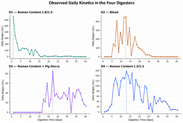
Figure 1 shows strongly differentiated profiles. (D1) produced 646 mL on the first day, representing 26.6% of its final cumulative volume, and then declined rapidly; production became zero after day 33. (D2) produced no gas during the first five days, reached a maximum of 453 mL on day 13, and then became zero after day 28. (D3) showed the longest lag: its first production appeared on day 17 and its peak of 84 mL occurred on day 22; 13 mL were still observed on day 40. (D4) started progressively, reached 156 mL on day 13, and maintained low production through the final day.

Source: Our calculations.

Download: Download full-size image

Figure 1. Observed daily kinetics in the four digesters.

The reconstructed cumulative volumes confirm the volumetric ranking of (D2), followed by (D4), (D1), and (D3). The empirical 90% threshold of final volume was crossed on days 13, 20, 37, and 31, respectively. For (D1), the final five days with no production satisfy the low-terminal-production criterion. (D2) was also stabilized before day 40. (D3) did not satisfy this criterion because production on day 40 still represented 1.64% of its cumulative volume; its asymptotic potential therefore remains more strongly extrapolated.

Table 2. Descriptive summary of the reconstructed series.

Digester	Final volume (mL/load)	Daily peak (mL)	Peak day	Empirical t90 (day)	Production on day 40 (% of cumulative)
D1	2,432	646	1	13	0.00
D2	3,415	453	13	20	0.00
D3	795	84	22	37	1.64
D4	2,492	156	13	31	0.32

Source: Our calculations from the audited daily data.

3.2. Model Comparison

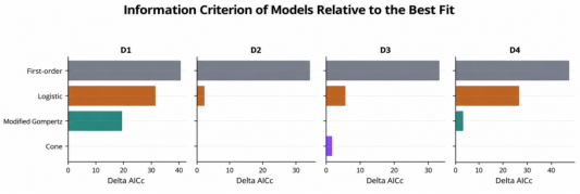
Table 3 compares the four structures. For daily residuals, the Cone model minimizes (AICc) for (D1) and (D4). The modified Gompertz model gives the minimum for (D2) and (D3). The cumulative R² values, ranging from 0.967 to 0.998 for the selected models, are systematically higher than daily

R^{2}

values, which range from 0.576 to 0.948. This difference illustrates precisely why an

R^{2}

calculated only from cumulative data is insufficient to validate a model.

Table 3. Comparative Model Performance for the Four Digesters.

Digester	Model	Daily RMSE (mL)	Daily R2	Cumulative RMSE (mL)	Cumulative R2	AICc	Delta AICc
D1	First-order	45.83	0.847	140.27	0.903	312.66	40.23
D1	Modified Gompertz	34.23	0.915	53.35	0.986	291.78	19.35
D1	Logistic	39.90	0.884	69.28	0.976	304.05	31.61
D1	Cone	26.87	0.948	82.15	0.967	272.44	0.00
D2	First-order	121.18	0.107	503.04	0.854	390.45	34.37
D2	Modified Gompertz	76.46	0.645	81.75	0.996	356.08	0.00
D2	Logistic	78.38	0.626	125.06	0.991	358.07	1.99
D2	Cone	76.51	0.644	83.44	0.996	356.13	0.05
D3	First-order	21.11	-0.035	172.94	0.623	250.65	33.20
D3	Modified Gompertz	13.52	0.576	26.15	0.991	217.45	0.00
D3	Logistic	14.49	0.512	54.52	0.963	223.04	5.59
D3	Cone	13.79	0.558	35.76	0.984	219.08	1.63
D4	First-order	45.92	0.101	214.71	0.940	312.81	47.46
D4	Modified Gompertz	25.55	0.721	53.63	0.996	268.41	3.06
D4	Logistic	34.18	0.502	166.25	0.964	291.66	26.32
D4	Cone	24.60	0.742	36.30	0.998	265.35	0.00

A zero Delta AICc denotes the minimum within each digester. The negative daily R² for D3 under the first-order model indicates a daily prediction less accurate than the observed mean.

Source: Our nonlinear least-squares fits.

As a reproducible check, for (D4) with the Cone model, the daily RMSE of 24.595 mL corresponds to RSS 40

\times {(24, 595)}^{2}

= 24197,5

m L^{2}

. With N = 40 and K = 4, substitution into the expression:

t_{90 / 40}

\inf {t : \hat{B} (t) \geq 0, 90 B_{obs} (40)}

, gives AICc = 265.35, the value reported in Table 3. Figure 2 makes the information differences visible; it also shows that (D2) presents near-equivalence between Gompertz and Cone, whose Akaike weights are 0.427 and 0.415, respectively.

Source: our calculations.

Download: Download full-size image

Figure 2. Information difference of each model relative to the best fit.

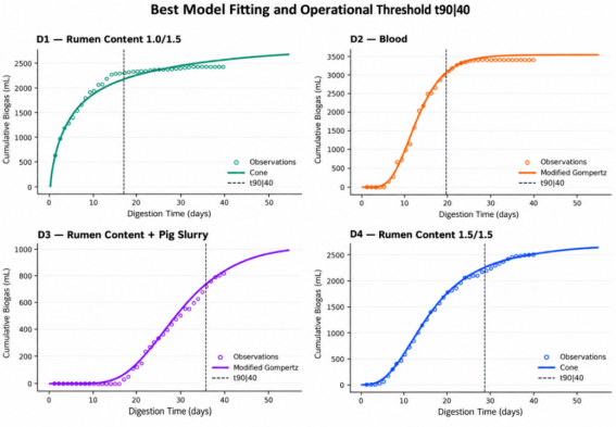
The fitted curves reproduce the general cumulative trajectory adequately (Figure 3). However, they should not conceal daily fluctuations, particularly the multiple peaks of (D2) and the late resurgence of (D3).

Source: Our calculations

Download: Download full-size image

Figure 3. Daily kinetics observed in the four digesters.

3.3. Kinetic Parameters and Uncertainty

Table 4. Parameters and Characteristic Times of the Selected Models.

Digester	Model	P (mL) [95% CI]	Specific parameters	t90 of P (d) [95% CI]	t90\|40 (d) [95% CI]
D1	Cone	3,110.4 [2,524.9-4,322.5]	kC = 0.17981; n = 0.78093	92.71 [33.84-393.38]*	16.84 [14.45-29.67]
D2	Modified Gompertz	3,538.9 [3,198.3-4,257.8]	Rmax = 298.16 mL/d; λ = 6.47 d	20.67 [18.99-23.36]	19.39 [16.78-22.53]
D3	Modified Gompertz	994.9 [787.2-1,417.1]	Rmax = 40.70 mL/d; λ = 16.82 d	46.05 [39.42-59.20]	35.80 [33.19-39.68]
D4	Cone	2,698.6 [2,413.9-3,053.0]	kC = 0.06379; n = 2.66479	35.75 [30.45-43.48]	28.53 [26.04-30.90]

Intervals are based on 1,000 moving-block bootstraps of daily residuals. * For D1,

t_{90}

of P is an unstable extrapolation and is not used for the operational decision.

Source: Our calculations.

The parameters of the selected models are summarized in Table 4. (D2) has a lag time of 6.47 days and an adjusted maximum rate of 298.16 mL/day. (D3) has a much longer lag time, 16.82 days, and a maximum rate seven times lower, 40.70 mL/day. For D4, the Cone shape parameter is greater than 1, producing an acceleration phase followed by deceleration consistent with its curve. For (D1), n is below 1; the mathematical slope near the origin becomes very steep and the extrapolated potential remains poorly identified despite the low daily RMSE.

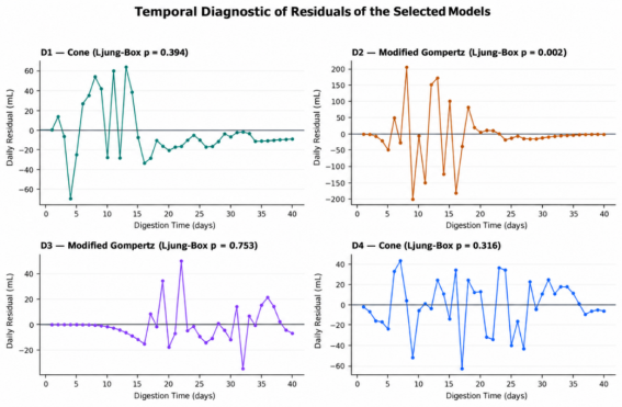
Residual diagnostics qualify the apparent quality of the cumulative fits. The Ljung-Box test detects no residual autocorrelation for (D1), (D3), and (D4) at conventional thresholds, with p = 0.394, 0.753, and 0.316. For (D2), p = 0.0019 and Durbin-Watson = 2.77 indicate temporal alternation not fully described by a single-phase sigmoid. Normality is rejected for (D1), (D2), and (D3) but not for (D4). Block bootstrap limits dependence on the normality assumption without eliminating the absence of replicates.

Source: our calculations.

Download: Download full-size image

Figure 4. Daily residuals of the selected kinetic models.

3.4. Energy Optimization of Cycle Duration

Table 5. Apparent energy balance and proposed cycle duration.

Digester	E40 (Wh/load)	t90\|40 (d)	E at t90\|40 (Wh)	Productivity (Wh/d)	Reduction vs 40 d (%)
D1	15.916	16.84	14.325	0.851	57.91
D2	23.174	19.39	20.857	1.075	51.51
D3	4.511	35.80	4.060	0.113	10.51
D4	16.309	28.53	14.678	0.515	28.74

E40 is apparent gross chemical energy per load, calculated using the CH₄ fractions from the source study and without correction to standard conditions.

Source: Our calculations.

Table 5 presents the energy translation. (D2) provides 23.174 Wh of apparent gross energy per load on day 40, 45.6% more than (D1) and 42.1% more than (D4). (D3) remains clearly lower at 4.511 Wh. At the

t_{90 / 40}

threshold, (D2) retains 20.857 Wh in 19.39 days and reaches the highest productivity, 1.075 Wh/day. (D1) reaches 14.325 Wh in 16.84 days and ranks second for cycle productivity. (D4) requires 28.53 days, whereas (D3) requires 35.80 days to recover only 4.060 Wh.

Source: our calculations.

Download: Download full-size image

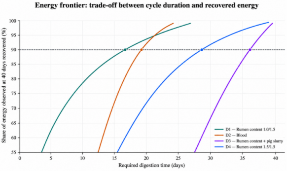
Figure 5. Energy-time frontier relative to the energy observed on day 40.

Figure 5 illustrates the trade-off between duration and recovered energy. The (D1) and (D2) curves rapidly reach the 90% region. (D4) follows an intermediate trajectory. (D3) shifts to the right, indicating long reactor occupancy for modest energy. Between 90% and 95%, each additional gain requires a disproportionate increase in duration; this supports choosing

t_{90 / 40}

as the decision threshold rather than systematically targeting 100%.

4. Discussion

4.1. Kinetic Interpretation of the Substrates

The best performance of (D2) is consistent with the high organic matter content of blood and its methane fraction of 68.27%. Its lag of nearly one week may reflect an adaptation phase before rapid conversion of biodegradable compounds. However, the presence of multiple peaks and negative residual autocorrelation suggests that a single sigmoid model does not represent all stages. A multiphasic function could reduce this residual structure, but it would add parameters that cannot be identified from a single series. The Gompertz choice therefore remains parsimonious and operational rather than mechanistic.

(D1) is characterized by immediate and very high production, with no observable lag. This shape favors the Cone model with n below 1 but makes its asymptotic potential fragile. The estimate of 3,110 mL exceeds the measured cumulative volume by 27.9%, although production is zero during the final days. This conflict between daily fit criterion and terminal plausibility justifies using

t_{90 / 40}

= 16.84 days rather than the asymptotic

t_{90}

of 92.71 days. It also demonstrates the value of combining AICc, residuals, terminal state, and biological interpretation, in line with previous comparisons

[18, 20, 21, 23]

(D4), more heavily loaded with rumen content than (D1), shows a gradual increase, production distributed across the cycle, and a

t_{90 / 40}

of 28.53 days. The descriptive (D1)-(D4) comparison suggests that stronger dilution accelerates energy recovery per unit time, whereas a more concentrated load maintains later production. This observation is consistent with the favorable effect of dilution reported for some slaughterhouse by-products

[26]

. It is not causal evidence, however, because (D1) and (D4) were not replicated and the actual volatile-matter concentration of the mixture was not calculated.

(D3) has the longest lag and the lowest potential. Production still active on day 40 explains why its P and asymptotic

t_{90}

are less well bounded. Co-digestion may improve nutrient balance, but its effect depends on proportions, inoculum, and inhibitors; it does not guarantee increased potential

[12, 14]

. Under the present conditions, the rumen-content-pig-slurry mixture shows no energy advantage over the mono-substrates. A controlled extension of the experiment, combined with replicates, would be necessary before concluding on its ultimate potential.

4.2. Scope of the Energy Optimization

The

t_{90 / 40}

threshold transforms a gas-production curve into a simple management rule: stop or renew a load when 90% of its reference energy has been recovered. Applied to the four tests, it substantially reduces duration for (D1) and (D2), more moderately for (D4), and only slightly for (D3). At constant reactor volume, a shorter duration theoretically allows more annual cycles. This reasoning concerns a laboratory batch reactor, however; in a semi-continuous household biodigester, hydraulic retention time, daily organic loading, and temperature must be considered simultaneously.

The proposed indicator is deliberately energy- and time-based. It includes neither substrate cost, energy consumed by the system, nor digestate stability. A net optimization should maximize useful energy after deducting heating, mixing, pumping, and losses, subject to constraints on pH, alkalinity, ammonia, and volatile fatty acids. Multi-objective formulations could then balance energy, time, cost, and pollution reduction. The present study provides the initial kinetic parameters required for this step, but not yet all of its variables.

At the local scale, priority given to (D2) should also be tempered by blood collection and sanitary safety, its high nitrogen content, and ammonia risk

[6, 16]

. (D1) may offer rapid start-up, whereas (D4) may be more suitable when supply is less frequent. The model therefore does not replace contextualized technical choice. It organizes the available options and identifies additional measurements that would reduce uncertainty.

4.3. Contribution to the Thesis and Implications for BioFaso 15

This analysis establishes a methodological link between assessment of slaughterhouse-waste potential and diagnosis of biodigesters installed in Forest Guinea. The

t_{90 / 40}

times, fitted rates, and residual profiles are parameters that can be directly compared with actual residence times, feeding frequencies, and gas volumes observed in BioFaso 15 units. A persistent difference between reference kinetics and on-site operation could direct the diagnosis toward overloading, insufficient temperature, inadequate dilution, or inhibition.

To move from descriptive decision support to numerical optimization of energy parameters, the next campaign should implement an experimental design with biological replicates. Minimum factors are organic loading, dilution, co-digestion ratio, and, if controllable, temperature. Responses should include CH₄ normalized per gram of volatile matter, Rmax,

t_{90}

, net energy, pH, alkalinity, volatile fatty acids, and ammonia. Response-surface or multi-objective optimization could then identify an operating domain rather than a single cycle time.

4.4. Limitations

Four main limitations frame the results. First, each treatment corresponds to a single series; bootstrap intervals do not quantify biological variability. Second, the absence of an inoculum blank, positive control, and normalization to standard conditions prevents the values from being qualified as normalized BMP values

[15, 16]

. Third, the CH₄ fraction is not documented day by day and its assignment to (D3) remains ambiguous; calculated energy is therefore conditional. Fourth, empirical models describe the curve without identifying hydrolysis, acidogenesis, or inhibition mechanisms. The results should not be extrapolated to other volumes or continuous operation without external validation.

5. Conclusions

Modeling daily production makes it possible to transform the N’Zérékoré slaughterhouse experiments into energy decision indicators. After auditing, the retained cumulative volumes are 2,432 mL for (D1), 3,415 mL for (D2), 795 mL for (D3), and 2,492 mL for (D4). The Cone and modified Gompertz models describe the (D1)-(D4) and (D2)-(D3) profiles, respectively, with the best AICc compromises.

At the operational

t_{90 / 40}

threshold, estimated durations are 16.84 days for (D1), 19.39 days for (D2), 35.80 days for (D3), and 28.53 days for (D4). (D2) provides the highest apparent gross energy under the tested conditions: 23.174 Wh on day 40 and 1.075 Wh/day at the threshold. (D1) provides the fastest recovery after smoothing, but its extrapolated asymptote is not sufficiently identifiable to guide the decision alone. (D3) combines a long lag with low energy, whereas (D4) occupies an intermediate position.

Thus, applying a uniform 40-day duration is not energetically appropriate for all loads. The

t_{90 / 40}

threshold provides a cautious and reproducible rule for adapting cycle duration. Validation on BioFaso 15 biodigesters will nevertheless require standardized measurements, replicates, monitoring of gas composition, and an accounting of energy consumed. Under these conditions, the temporal optimization presented here can evolve toward causal and multi-objective optimization of energy parameters in Forest Guinea.

Abbreviations

AD	Anaerobic Digestion
AIC	Akaike Information Criterion
AICc	Corrected Akaike Information Criterion
BMP	Biochemical Methane Potential
CI	Confidence Interval
D	Digester
LCFAs	Long-chain Fatty Acids
MAE	Mean Absolute Error
RMSE	Root Mean Square Error
UASB	Upflow Anaerobic Sludge Blanket

Acknowledgments

The authors thank the managers and staff of the N’Zérékoré slaughterhouse for access to the site and organic materials during the initial experimental campaign.

Author Contributions

Faya Maurice Yombouno: Conceptualization, Data curation, Formal Analysis, Investigation, Methodology, Software, Validation, Visualization, Writing – original draft, Writing – review & editing

Toha François Lihonou: Conceptualization, Data curation, Formal Analysis, Investigation, Methodology, Software, Validation, Visualization, Writing – original draft, Writing – review & editing

Ansoumane Sakouvogui: Data curation, Formal Analysis, Software, Validation, Visualization

Ibrahima Bayo: Investigation, Validation, Visualization, Writing – original draft, Writing – review & editing

Nakany Camara: Supervision, Validation, Writing – review & editing

Salifou Tera: Supervision, Validation, Writing – review & editing

Data Availability Statement

The daily biogas production data used for model fitting are reproduced in full in Appendix A. Additional information concerning experimental conditions, physicochemical measurements, and measurement procedures is available from the authors upon reasonable request.

Conflicts of Interest

The authors declare no conflicts of interest.

Appendix: Audited Daily Data Used for Modelling

Table 6. Daily biogas production by digester.

Day	D1 (mL)	D2 (mL)	D3 (mL)	D4 (mL)
1	646	0	0	0
2	334	0	0	3
3	216	0	0	6
4	98	0	0	20
5	109	0	0	30
6	138	143	0	104
7	129	120	0	131
8	135	409	0	107
9	112	49	0	64
10	33	277	0	120
11	115	147	0	132
12	20	447	0	129
13	109	453	0	156
14	79	133	0	139
15	29	330	0	109
16	0	16	0	150
17	2	130	27	46
18	18	224	21	125
19	10	137	60	105
20	4	102	12	98
21	6	91	26	46
22	5	75	84	37
23	10	53	33	100
24	14	25	38	92
25	8	22	31	13
26	0	21	27	32
27	0	8	30	0
28	4	3	41	62
29	11	0	35	31
30	7	0	26	43
31	11	0	50	54
32	11	0	0	38
33	9	0	39	42
34	0	0	30	40
35	0	0	44	32
36	0	0	47	20
37	0	0	39	8
38	0	0	25	10
39	0	0	17	10
40	0	0	13	8
Total	2 432	3 415	795	2 492

Source: Workbook incorporated into Yombouno et al.

[1]

; blank cells were converted to zeros without modifying the numerical daily values.

References

[1]	L. Appels, J. Baeyens, J. Degrève, R. Dewil, “Principles and potential of the anaerobic digestion of waste-activated sludge,” Progress in Energy and Combustion Science, 34(6), 755-781, 2008. https://doi.org/10.1016/j.pecs.2008.06.002
[2]	P. Weiland, “Biogas production: Current state and perspectives,” Applied Microbiology and Biotechnology, 85(4), 849-860, 2010. https://doi.org/10.1007/s00253-009-2246-7
[3]	D. J. Batstone, J. Keller, I. Angelidaki, S. V. Kalyuzhnyi, S. G. Pavlostathis, A. Rozzi, W. T. M. Sanders, H. Siegrist, V. A. Vavilin, “The IWA anaerobic digestion model No. 1 (ADM1),” Water Science and Technology, 45(10), 65-73, 2002. https://doi.org/10.2166/wst.2002.0292
[4]	J. Palatsi, M. Viñas, M. Guivernau, B. Fernandez, X. Flotats, “Anaerobic digestion of slaughterhouse waste: Main process limitations and microbial community interactions,” Bioresource Technology, 102(3), 2219-2227, 2011. https://doi.org/10.1016/j.biortech.2010.09.121
[5]	Z. Ning, H. Zhang, W. Li, R. Zhang, G. Liu, C. Chen, “Anaerobic digestion of lipid-rich swine slaughterhouse waste: Methane production performance, long-chain fatty acids profile and predominant microorganisms,” Bioresource Technology, 269, 426-433, 2018. https://doi.org/10.1016/j.biortech.2018.08.001
[6]	Y. Chen, J. J. Cheng, K. S. Creamer, “Inhibition of anaerobic digestion process: A review,” Bioresource Technology, 99(10), 4044-4064, 2008. https://doi.org/10.1016/j.biortech.2007.01.057
[7]	I. Ruiz, M. C. Veiga, P. de Santiago, R. Blazquez, “Treatment of slaughterhouse wastewater in a UASB reactor and an anaerobic filter,” Bioresource Technology, 60(3), 251-258, 1997. https://doi.org/10.1016/S0960-8524(97)00020-5
[8]	A. D. Shende, G. R. Pophali, “Anaerobic treatment of slaughterhouse wastewater: A review,” Environmental Science and Pollution Research, 28(1), 35-55, 2021. https://doi.org/10.1007/s11356-020-10921-x
[9]	R. Borja, C. J. Banks, Z. Wang, “Anaerobic digestion of slaughterhouse wastewater using a combination sludge blanket and filter arrangement in a single reactor,” Bioresource Technology, 65(1-2), 125-133, 1998. https://doi.org/10.1016/S0960-8524(98)00004-2
[10]	A. J. Ward, P. J. Hobbs, P. J. Holliman, D. L. Jones, “Optimisation of the anaerobic digestion of agricultural resources,” Bioresource Technology, 99(17), 7928-7940, 2008. https://doi.org/10.1016/j.biortech.2008.02.044
[11]	B. Drosg, Process Monitoring in Biogas Plants, IEA Bioenergy, Task 37, 2013. https://task37.ieabioenergy.com/technical-reports/process-monitoring-in-biogas-plants/
[12]	J. Mata-Alvarez, J. Dosta, M. S. Romero-Güiza, X. Fonoll, M. Peces, S. Astals, “A critical review on anaerobic co-digestion achievements between 2010 and 2013,” Renewable and Sustainable Energy Reviews, 36, 412-427, 2014. https://doi.org/10.1016/j.rser.2014.04.039
[13]	S. A. Neshat, M. Mohammadi, G. D. Najafpour, P. Lahijani, “Anaerobic co-digestion of animal manures and lignocellulosic residues as a potent approach for sustainable biogas production,” Renewable and Sustainable Energy Reviews, 79, 308-322, 2017. https://doi.org/10.1016/j.rser.2017.05.137
[14]	S. Astals, D. J. Batstone, S. Tait, P. D. Jensen, “Identification of synergistic impacts during anaerobic co-digestion of organic wastes,” Bioresource Technology, 169, 421-427, 2014. https://doi.org/10.1016/j.biortech.2014.07.024
[15]	I. Angelidaki, D. Karakashev, D. J. Batstone, C. M. Plugge, A. J. M. Stams, “Defining the biomethane potential (BMP) of solid organic wastes and energy crops: A proposed protocol for batch assays,” Water Science and Technology, 59(5), 927-934, 2009. https://doi.org/10.2166/wst.2009.040
[16]	C. Holliger, M. Alves, D. Andrade, I. Angelidaki, S. Astals, U. Baier, C. Bougrier, P. Buffière, M. Carballa, V. de Wilde, F. Ebertseder, B. Fernández, E. Ficara, I. Fotidis, J.-C. Frigon, H. F. de Laclos, D. S. M. Ghasimi, G. Hack, M. Hartel, et al., “Towards a standardization of biomethane potential tests,” Water Science and Technology, 74(11), 2515-2522, 2016. https://doi.org/10.2166/wst.2016.336
[17]	C. Holliger, S. Astals, H. F. de Laclos, S. D. Hafner, K. Koch, S. Weinrich, “Towards a standardization of biomethane potential tests: A commentary,” Water Science and Technology, 83(1), 247-250, 2021. https://doi.org/10.2166/wst.2020.569
[18]	H. M. El-Mashad, “Kinetics of methane production from the codigestion of switchgrass and Spirulina platensis algae,” Bioresource Technology, 132, 305-312, 2013. https://doi.org/10.1016/j.biortech.2012.12.183
[19]	F. Raposo, M. A. De la Rubia, V. Fernández-Cegrí, R. Borja, “Anaerobic digestion of solid organic substrates in batch mode: An overview relating to methane yields and experimental procedures,” Renewable and Sustainable Energy Reviews, 16(1), 861-877, 2012. https://doi.org/10.1016/j.rser.2011.09.008
[20]	D. D. Nguyen, B.-H. Jeon, J. H. Jeung, E. R. Rene, J. R. Banu, B. Ravindran, C. M. Vu, H. H. Ngo, W. Guo, S. W. Chang, “Thermophilic anaerobic digestion of model organic wastes: Evaluation of biomethane production and multiple kinetic models analysis,” Bioresource Technology, 280, 269-276, 2019. https://doi.org/10.1016/j.biortech.2019.02.033
[21]	H. Akaike, “A new look at the statistical model identification,” IEEE Transactions on Automatic Control, 19(6), 716-723, 1974. https://doi.org/10.1109/TAC.1974.1100705
[22]	C. M. Hurvich, C.-L. Tsai, “Regression and time series model selection in small samples,” Biometrika, 76(2), 297-307, 1989. https://doi.org/10.1093/biomet/76.2.297
[23]	N. W. S. Morais, M. M. H. Coelho, A. de S. E. Silva, F. S. S. Silva, T. J. T. Ferreira, E. L. Pereira, A. B. dos Santos, “Biochemical potential evaluation and kinetic modeling of methane production from six agro-industrial wastewaters in mixed culture,” Environmental Pollution, 280, 116876, 2021. https://doi.org/10.1016/j.envpol.2021.116876
[24]	D. Deublein, A. Steinhauser, Biogas from Waste and Renewable Resources: An Introduction, 2nd revised and expanded ed., Wiley-VCH, 2011. https://doi.org/10.1002/9783527632794
[25]	F. M. Yombouno, I. Bayo, P. Summy, O. Keita &. Agbazo, “Evaluation of methane potential of slaughterhouse waste in the urban municipality of N'Zérékoré, Guinea Republic”, Research Journal of Physical Sciences, 14(2), 1-8. https://www.isca.me/PHY_SCI/Archive/v14/i2/1.ISCA-RJPS-2025-003.php
[26]	J.-J. Lay, Y.-Y. Li, T. Noike, “Influences of pH and moisture content on the methane production in high-solids sludge digestion,” Water Research, 31(6), 1518-1524, 1997. https://doi.org/10.1016/S0043-1354(96)00413-7
[27]	R. Karki, W. Chuenchart, K. C. Surendra, S. Sung, L. Raskin, S. K. Khanal, “Anaerobic co-digestion of various organic wastes: Kinetic modeling and synergistic impact evaluation,” Bioresource Technology, 343, 126063, 2022. https://doi.org/10.1016/j.biortech.2021.126063
[28]	B. Efron, R. Tibshirani, “Bootstrap methods for standard errors, confidence intervals, and other measures of statistical accuracy,” Statistical Science, 1(1), 54-75, 1986. https://doi.org/10.1214/ss/1177013815
[29]	M. H. Zwietering, I. Jongenburger, F. M. Rombouts, K. van ’t Riet, “Modeling of the bacterial growth curve,” Applied and Environmental Microbiology, 56(6), 1875-1881, 1990. https://doi.org/10.1128/AEM.56.6.1875-1881.1990

Cite This Article

Plain Text BibTeX RIS

APA Style

Yombouno, F. M., Lihonou, T. F., Sakouvogui, A., Bayo, I., Camara, N., et al. (2026). Kinetic Modeling and Energy Optimization of Biogas Production from Slaughterhouse Waste in Forest Guinea. Science Journal of Energy Engineering, 14(4), 98-111. https://doi.org/10.11648/j.sjee.20261404.11

Copy | Download

ACS Style

Yombouno, F. M.; Lihonou, T. F.; Sakouvogui, A.; Bayo, I.; Camara, N., et al. Kinetic Modeling and Energy Optimization of Biogas Production from Slaughterhouse Waste in Forest Guinea. Sci. J. Energy Eng. 2026, 14(4), 98-111. doi: 10.11648/j.sjee.20261404.11

Copy | Download

AMA Style

Yombouno FM, Lihonou TF, Sakouvogui A, Bayo I, Camara N, et al. Kinetic Modeling and Energy Optimization of Biogas Production from Slaughterhouse Waste in Forest Guinea. Sci J Energy Eng. 2026;14(4):98-111. doi: 10.11648/j.sjee.20261404.11

Copy | Download

@article{10.11648/j.sjee.20261404.11,
  author = {Faya Maurice Yombouno and Toha François Lihonou and Ansoumane Sakouvogui and Ibrahima Bayo and Nakany Camara and Salifou Tera},
  title = {Kinetic Modeling and Energy Optimization of Biogas Production from Slaughterhouse Waste in Forest Guinea},
  journal = {Science Journal of Energy Engineering},
  volume = {14},
  number = {4},
  pages = {98-111},
  doi = {10.11648/j.sjee.20261404.11},
  url = {https://doi.org/10.11648/j.sjee.20261404.11},
  eprint = {https://article.sciencepublishinggroup.com/pdf/10.11648.j.sjee.20261404.11},
  abstract = {Anaerobic digestion of slaughterhouse waste can mitigate pollution while supplying locally usable energy. Final biogas volume alone, however, does not define a rational operating time. This study modeled daily kinetics from four experimental loads monitored for 40 days in N’Zérékoré: diluted rumen content (D1), blood (D2), rumen content-pig slurry (D3), and a more concentrated rumen-content treatment (D4). First-order, modified Gompertz, logistic, and Cone models were fitted by nonlinear least squares to daily increments and compared using corrected Akaike information criterion, RMSE, MAE, , and residual diagnostics. Fitting uncertainty was assessed using 1,000 moving-block bootstrap repl icates. An operational threshold,, was defined as the modeled time required to recover 90% of the biogas energy observed on day 40. Recalculated cumulative volumes were 2,432, 3,415, 795, and 2,492 mL per experimental load for (D1)-(D4). The Cone model was selected for (D1) and (D4), whereas the modified Gompertz model best described (D2) and (D3). Estimated  values were 16.84, 19.39, 35.80, and 28.53 days, respectively. Using methane fractions reported in the source study and a methane lower heating value of 9.94 kWh/, apparent gross energies were 15.92, 23.17, 4.51, and 16.31 Wh per load. (D2) combined the highest total energy with an energy productivity of 1.075 Wh/day at . The proposed operating times would shorten digester occupancy by 57.9%, 51.5%, 10.5%, and 28.7% relative to a fixed 40-day cycle. These estimates provide a numerical decision aid for cycle duration, rather than causal optimization of operating variables, because the dataset includes no biological replicates, blank controls, or factorial design.},
 year = {2026}
}

Copy | Download

TY - JOUR
T1 - Kinetic Modeling and Energy Optimization of Biogas Production from Slaughterhouse Waste in Forest Guinea
AU - Faya Maurice Yombouno
AU - Toha François Lihonou
AU - Ansoumane Sakouvogui
AU - Ibrahima Bayo
AU - Nakany Camara
AU - Salifou Tera
Y1 - 2026/10/26
PY - 2026
N1 - https://doi.org/10.11648/j.sjee.20261404.11
DO - 10.11648/j.sjee.20261404.11
T2 - Science Journal of Energy Engineering
JF - Science Journal of Energy Engineering
JO - Science Journal of Energy Engineering
SP - 98
EP - 111
PB - Science Publishing Group
SN - 2376-8126
UR - https://doi.org/10.11648/j.sjee.20261404.11
AB - Anaerobic digestion of slaughterhouse waste can mitigate pollution while supplying locally usable energy. Final biogas volume alone, however, does not define a rational operating time. This study modeled daily kinetics from four experimental loads monitored for 40 days in N’Zérékoré: diluted rumen content (D1), blood (D2), rumen content-pig slurry (D3), and a more concentrated rumen-content treatment (D4). First-order, modified Gompertz, logistic, and Cone models were fitted by nonlinear least squares to daily increments and compared using corrected Akaike information criterion, RMSE, MAE, , and residual diagnostics. Fitting uncertainty was assessed using 1,000 moving-block bootstrap repl icates. An operational threshold,, was defined as the modeled time required to recover 90% of the biogas energy observed on day 40. Recalculated cumulative volumes were 2,432, 3,415, 795, and 2,492 mL per experimental load for (D1)-(D4). The Cone model was selected for (D1) and (D4), whereas the modified Gompertz model best described (D2) and (D3). Estimated values were 16.84, 19.39, 35.80, and 28.53 days, respectively. Using methane fractions reported in the source study and a methane lower heating value of 9.94 kWh/, apparent gross energies were 15.92, 23.17, 4.51, and 16.31 Wh per load. (D2) combined the highest total energy with an energy productivity of 1.075 Wh/day at . The proposed operating times would shorten digester occupancy by 57.9%, 51.5%, 10.5%, and 28.7% relative to a fixed 40-day cycle. These estimates provide a numerical decision aid for cycle duration, rather than causal optimization of operating variables, because the dataset includes no biological replicates, blank controls, or factorial design.
VL - 14
IS - 4
ER -

Copy | Download

Author Information

Faya Maurice Yombouno

Department of Physics, University of N’Zerekore, N’Zerekore, Guinea

Contact Email

http://orcid.org/0009-0001-4540-2842
Toha François Lihonou

Department of Physics, University of N’Zerekore, N’Zerekore, Guinea;Laboratory of Fluid Mechanics, Nonlinear Dynamics and Modeling of Biological Systems (LMFDNMSB), Institute of Mathematics and Physical Sciences, Porto-Novo, Benin

Contact Email

http://orcid.org/0009-0003-3144-3285
Ansoumane Sakouvogui

Department of Physics, Higher Institute of Technology, Mamou, Guinea

Contact Email

http://orcid.org/0000-0001-7619-0566
Ibrahima Bayo

Marine and Coastal Research Centre (CEREMAC), UGANC, Conakry, Guinea

Contact Email

http://orcid.org/0009-0004-4697-5433
Nakany Camara

Department of Physics, University of N’Zerekore, N’Zerekore, Guinea

Contact Email
Salifou Tera

Department of Physics, University of N’Zerekore, N’Zerekore, Guinea

Contact Email

http://orcid.org/0009-0006-1376-6277

Download PDF

Submit an Article

Abstract
Keywords
Document Sections
Show Full Outline
Abbreviations
Acknowledgments
Author Contributions
Data Availability Statement
Conflicts of Interest
Appendix: Audited Daily Data Used for Modelling
References
Cite This Article
Author Information

Plain Text BibTeX RIS

APA Style

Yombouno, F. M., Lihonou, T. F., Sakouvogui, A., Bayo, I., Camara, N., et al. (2026). Kinetic Modeling and Energy Optimization of Biogas Production from Slaughterhouse Waste in Forest Guinea. Science Journal of Energy Engineering, 14(4), 98-111. https://doi.org/10.11648/j.sjee.20261404.11

Copy | Download

ACS Style

Yombouno, F. M.; Lihonou, T. F.; Sakouvogui, A.; Bayo, I.; Camara, N., et al. Kinetic Modeling and Energy Optimization of Biogas Production from Slaughterhouse Waste in Forest Guinea. Sci. J. Energy Eng. 2026, 14(4), 98-111. doi: 10.11648/j.sjee.20261404.11

Copy | Download

AMA Style

Yombouno FM, Lihonou TF, Sakouvogui A, Bayo I, Camara N, et al. Kinetic Modeling and Energy Optimization of Biogas Production from Slaughterhouse Waste in Forest Guinea. Sci J Energy Eng. 2026;14(4):98-111. doi: 10.11648/j.sjee.20261404.11

Copy | Download

@article{10.11648/j.sjee.20261404.11,
  author = {Faya Maurice Yombouno and Toha François Lihonou and Ansoumane Sakouvogui and Ibrahima Bayo and Nakany Camara and Salifou Tera},
  title = {Kinetic Modeling and Energy Optimization of Biogas Production from Slaughterhouse Waste in Forest Guinea},
  journal = {Science Journal of Energy Engineering},
  volume = {14},
  number = {4},
  pages = {98-111},
  doi = {10.11648/j.sjee.20261404.11},
  url = {https://doi.org/10.11648/j.sjee.20261404.11},
  eprint = {https://article.sciencepublishinggroup.com/pdf/10.11648.j.sjee.20261404.11},
  abstract = {Anaerobic digestion of slaughterhouse waste can mitigate pollution while supplying locally usable energy. Final biogas volume alone, however, does not define a rational operating time. This study modeled daily kinetics from four experimental loads monitored for 40 days in N’Zérékoré: diluted rumen content (D1), blood (D2), rumen content-pig slurry (D3), and a more concentrated rumen-content treatment (D4). First-order, modified Gompertz, logistic, and Cone models were fitted by nonlinear least squares to daily increments and compared using corrected Akaike information criterion, RMSE, MAE, , and residual diagnostics. Fitting uncertainty was assessed using 1,000 moving-block bootstrap repl icates. An operational threshold,, was defined as the modeled time required to recover 90% of the biogas energy observed on day 40. Recalculated cumulative volumes were 2,432, 3,415, 795, and 2,492 mL per experimental load for (D1)-(D4). The Cone model was selected for (D1) and (D4), whereas the modified Gompertz model best described (D2) and (D3). Estimated  values were 16.84, 19.39, 35.80, and 28.53 days, respectively. Using methane fractions reported in the source study and a methane lower heating value of 9.94 kWh/, apparent gross energies were 15.92, 23.17, 4.51, and 16.31 Wh per load. (D2) combined the highest total energy with an energy productivity of 1.075 Wh/day at . The proposed operating times would shorten digester occupancy by 57.9%, 51.5%, 10.5%, and 28.7% relative to a fixed 40-day cycle. These estimates provide a numerical decision aid for cycle duration, rather than causal optimization of operating variables, because the dataset includes no biological replicates, blank controls, or factorial design.},
 year = {2026}
}

Copy | Download